What is a Queuing System? A flow of customers from a finite / infinite population towards your service facility forms a queue on account of lack of capability to serve them all at the same time. To manage this, you must have a queue system that consists of customers arriving for service, waiting for service if it is not immediate, and leaving the system after being served.
 In order to provide better customer service, you need to make your queues move faster. But first you need to know the current metrics of your queue system, including the average waiting time of a customer in a queue, and the total time the customer has to spend in the system.
There is a complete explanation of queuing theory below, along with the characteristics, math and formulas that you need to calculate these factors. But if you simply want to calculate the average waiting time your customers are facing, make use of this M/M/1 queuing theory calculator below.
Elements of queuing system
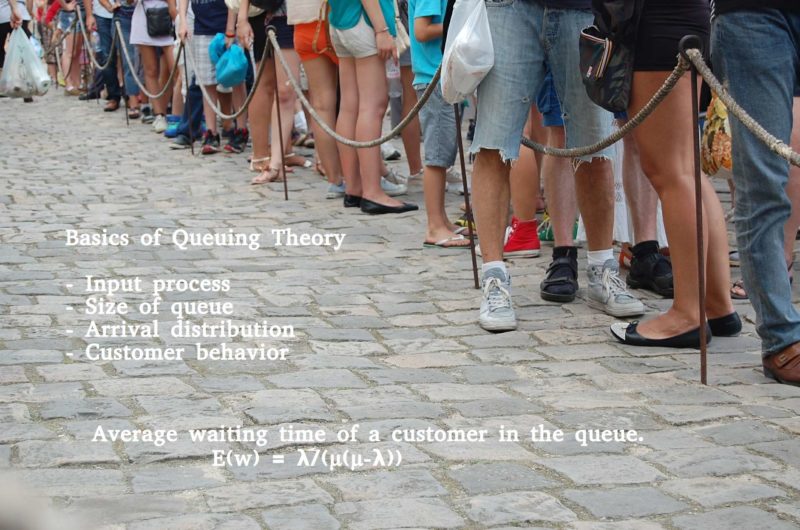
Input process – The pattern in which customers arrive in the system.
Size of the queue – The size of the input service is either finite or infinite.
Arrival distribution – The pattern in which the customers arrive at the service system or inter arrival time – The most common stochastic models arrival rate Poisson distribution and/or the inter arrival times follow exponential distribution.
Customer’s behaviour – The customer may wait in the queue whatever be the length of the queue or the customer leave the queue looking at the length of the queue.
Queue discipline
FIFO – First in first out
FCFS- First come first served
LIFO – Last in First out
Service mechanism
Single queue and one server
Single queue and several servers
Several queues and one server
Several servers.
Capacity of the queuing system
A finite source limits the customers arriving for service and infinite source is forever abundant.
Operating Characteristic of queuing system
Expected number of customers in the system E(n) or L
Expected number of customers in the Queue E(m) or Lq
Expected waiting line in the system W
Expected waiting time in the queue Wq
The service utilisation factor P = λ/µ: the proportion pf time that a server actually spends with a customer where, λ is the average number of customers arriving per unit of time and µ is the average number of customers completing the service per unit time.
Probability distributions in the queuing system
The models in which only arrival are counted is a pure birth models. In queuing theory is a birth-death processes because the additional customers increases the arrivals in the system and decreases by departure of serviced customers from the system
Distribution of arrivals:
Let Pn(t) be the probability of n arrivals in a time interval of length t, n ≥ 0 is an integer.
The arrival distribution is assumed as Poisson process with mean λt and the distribution is given by
Pn(t) = (λt)nexp(-λt)/n! , n ≥ 0
Here the random variable is defined as the number of arrivals to a system in time has the Poisson distribution with mean λt or mean arrival rate λ.
Distribution of inter arrival times:
Inter arrival time is defined as the time intervals between two successive arrivals. If the arrival process has the Poisson distribution then the random variable that is the time between successive arrivals follows an exponential distribution given by
f(t) = λexp(-λt), t ≥ 0.
Distribution of departures:
The queuing system starts with N customers at time t= 0 where N ≥ 0. Departures occurs at the rate of µ customers per unit time. Let Pn(t) be the probability that n customers remaining after t time units.
The probability distribution is stated below which is the Truncated Poisson distribution
Pn(t) = (µt)N-n exp(-µt)/(N-n), 1≤n≤N
P0(t) = 1- 1NPn(t)
Distribution of service times:
The probability for completing the service of n customers in time t has the exponential distribution with
s(t) = µexp(-µt) , t ≥ 0.
Classification of Queuing Models
The queuing model may be completely described by ( a/b/c)d/e)
a: inter arrival time distribution
b: distribution of inter service time
c: the number of servers in the system
d: capacity of the system
e: queue discipline
Model 1 (M/M/1):(∞/FIFO)
In this model queuing system has single server channel, Poisson input, exponential service, and there is no limit on the system capacity and customers are served on a first in first out basis.
Characteristics of the model:
Probability of queue size being greater than the number of customers is given by ρn, where ρ =λ/µ.
Average number of customers in the system
E(n) = λ/(µ-λ)=ρ/(1-ρ)
Average queue length is given by
E(m) = ρ2/(1-ρ). m= n-1, being the number of customers in the queue excluding the customer in service.
Average length of the nonempty queue
E(m│m>0) = ρ2
Average waiting time of a customer in the queue.
E(w) = λ/(µ(µ-λ))
Let the random variable v denote the total time that a customer has to spend in the system including the service.
E(v) = 1/(µ -λ)
This explanation of queuing theory and the associated math and formulas for calculating the average wait time within queue systems has been published with input from Prof. Dr. Rajalakshmi Padmanabhan , Head of Statistics, Bangalore University.
November 22nd, 2017 ·